For an interactive study of the phenomena discussed in this post, click here.
Signals — both waveforms across an analog line and the kind we use for distributed software observability — have formally characterizable properties. In fact, they share a name because in many respects they have the same formally characterizable properties. If we model the software systems we design as continuous, we can apply precisely the same mathematics to our systems that we do to analog signals. This is not merely a novelty. We can use the analytical and formal tools of signals processing to not only better understand our systems, but to create better designs and more correctly locate design and engineering responsibility.
Case study 1: a memory pulse, smeared
Imagine a service that gives traders a live view into the top 50 most volatile options contracts over the last hour. You already have a data pipe streaming firehose trade data into a fast, efficient store. On a regular clock, your service samples the last hour’s worth of trades into memory, performs a fast volatility calculation, and writes the volatility scores back to memory, ready to be picked up and served to traders who want it.
Because this is finance, deterministic compute matters. Each trade is represented as a dense struct, with no pointers. Something like:
type TradeEvent struct {
    Timestamp int64    // 8 bytes (Unix nanoseconds)
    Price     float64  // 8 bytes
    Size      int32    // 4 bytes
    Exchange  uint8    // 1 byte
    _         [3]byte  // 3 bytes (memory alignment padding)
    Symbol    [24]byte // 24 bytes (e.g., "AAPL  260515C00180000")
}
At peak trading hours the firehose runs around 7,000 trades/second. Do a little arithmetic, and that means your volatility compute service allocates just over a gigabyte on its regular tick, computes on that, and then releases the memory.
This is what your memory footprint really looks like:
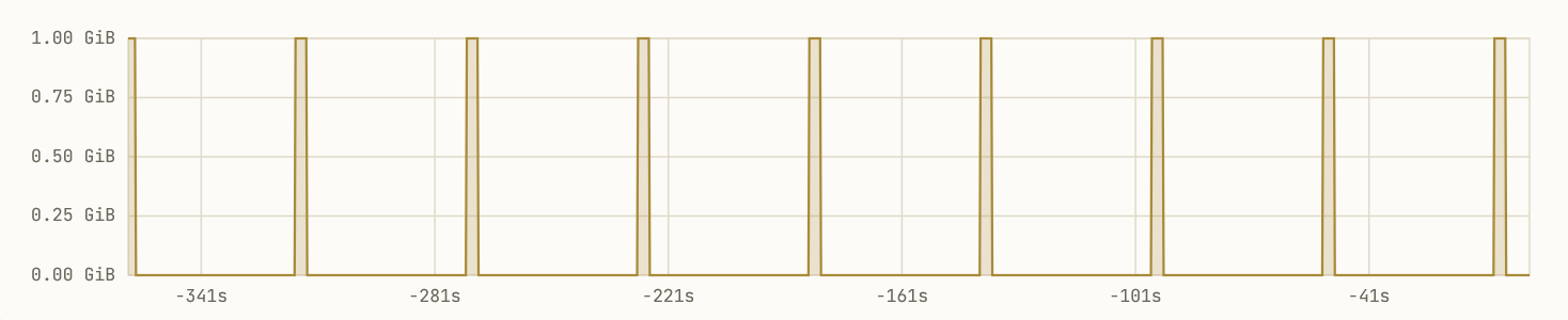
But this is what your SRE sees:
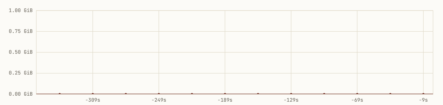
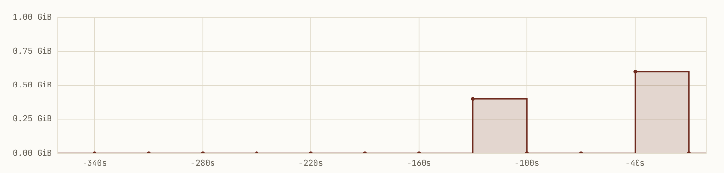
Dead flat for twelve real allocation cycles, then two peaks near each other that are both different and incorrect magnitudes.
What’s happening here?
What the SRE sees, and why
The standard SRE framing of this is sample rate aliasing, and it isn’t wrong — but it’s coarser than the situation deserves, and the coarseness is exactly what makes problems like this hard to design around. Let’s be precise.
The service runs every 44 seconds and holds its allocation for 3 seconds. The observability stack scrapes every 30 seconds and reports the mean over a 5-second integration window. Two distinct things are going wrong, and they compound.
The first is that the integration window is shorter than the pulse but on the same order of magnitude, which means each scrape that does land on a pulse catches some partial fraction of it — between zero and three seconds of the 3-second pulse, averaged over a 5-second window. The reported magnitude is therefore the pulse height scaled by (overlap / window), which can land anywhere from ~0 to ~600 MiB depending on phase alignment. This is amplitude smearing, and it’s why the two visible peaks are different magnitudes and both wrong.
The second is that the scrape interval and the pulse period have an unhelpful relationship. LCM(30, 44) = 660 seconds, so the entire sampling pattern repeats every eleven minutes. Inside each cycle, the 5-second window only intersects the 3-second pulse a couple of times, clustered near each other in phase, and then the sampler runs silent for the rest of the cycle. This is LCM clustering, and it’s why two peaks near each other are followed by long flat regions — not because the system is quiet, but because the sampler is.
Twelve flat scrapes followed by two wrong-magnitude peaks is the visible signature of these two pathologies stacking. Neither is exotic. Both are predictable from the parameters alone.
Case study 2: a ghost oscillation
The smearing case is bad because it makes a real signal look like noise. The next case is worse, because it makes a real signal look like a different real signal.
Consider a node running a periodic batch job: every 4 seconds, a worker spins up, drives CPU utilization to ~80% for about two seconds, then idles. Strictly periodic, well-behaved, exactly the kind of workload you might run in a tight scheduling loop. Now imagine your node exporter scrapes CPU utilization every 5 seconds, point-sampled — no integration window, just an instantaneous read of the counter at scrape time. This is closer to default behavior than most operators realize; many CPU and load metrics are functionally point samples even when the surrounding scrape claims a window.
Do the arithmetic. The workload has fundamental frequency f₀ = 1/4 = 0.25 Hz, with harmonics at 0.5 Hz, 0.75 Hz, and so on. The sampler runs at fₛ = 1/5 = 0.2 Hz, giving a Nyquist frequency of 0.1 Hz. Every component of the real signal is above Nyquist. With no integration window, nothing is filtered before sampling, and every harmonic folds:
- f₀ = 0.25 Hz folds to |0.25 − 0.2| = 0.05 Hz, apparent period 20 s
- 2f₀ = 0.5 Hz folds to |0.5 − 2·0.2| = 0.1 Hz, sitting right at Nyquist
- 3f₀ = 0.75 Hz folds to |0.75 − 4·0.2| = 0.05 Hz, reinforcing the fundamental’s alias
What the dashboard shows is a clean, low-frequency oscillation with an apparent period of roughly twenty seconds, riding on whatever baseline the node is otherwise doing. It looks like a real cycle. It is plausible enough that an experienced SRE will reach for explanations — a 20-second cron, a connection-pool refresh, a stats flush — none of which exist. The actual workload’s 4-second period is nowhere on the dashboard, and no amount of staring at the time series will recover it. The FFT of the sampler output will show a clean peak at 0.05 Hz with reinforcement from the third harmonic, and the FFT of the underlying signal will show peaks at 0.25, 0.5, 0.75 Hz that have no representation in what was sampled.
This is harmonic folding in its textbook form. It is the failure mode the Shannon-Nyquist theorem was written to describe.
The two case studies share a structure but fail differently. The memory pulse case produces a ragged signal — a few partial captures separated by long flat regions — because the integration window did some filtering, just not enough, and the LCM relationship clustered what little signal got through. The CPU case produces a clean signal — a smooth oscillation at a frequency the system does not physically generate — because no filtering happened at all, and the harmonics folded coherently into the baseband. Ragged data looks like a problem. Clean data looks like an answer. The clean version is more dangerous.
The deeper principle
Both case studies — the smeared pulse and the ghost oscillation — are surface expressions of the same underlying constraint: the Shannon-Nyquist sampling theorem. A continuous signal can be perfectly reconstructed from its samples if and only if the signal is bandlimited to some frequency B and the sample rate exceeds 2B. Below that rate, frequency components above the Nyquist limit fₛ/2 don’t disappear — they fold into the baseband at |f mod fₛ|, indistinguishable from genuine low-frequency content. The reconstruction is wrong, and worse, it’s wrong in a way that looks plausible.
Neither pulse train is bandlimited. A periodic pulse of width τ and period T decomposes into a Fourier series with components at every integer multiple of f₀ = 1/T, with amplitudes that fall off as sinc(kτ/T) but never vanish. The memory-allocation signal has meaningful spectral content well past 1 Hz; the CPU workload similarly. No 5-to-30-second sampler can capture either honestly. Both signals are, in the strict signals-theoretic sense, unsampleable at those rates.
The integration window is the only thing that saves us from total chaos, and it’s a double-edged tool. A non-zero window acts as a sinc-shaped low-pass filter applied before sampling: it attenuates content above roughly 1/window before that content can alias. With a window much greater than the pulse period, the signal converges to its duty-cycle-weighted DC mean (about 70 MiB, in our case) — the pulse structure is gone, but at least the dashboard isn’t lying about a flat steady-state load. With a window much shorter than the pulse period and a sample interval comparable to the period, you get the worst of both worlds: insufficient anti-alias filtering and insufficient sample density, producing amplitude-smeared point captures that look like noise or rare outliers when the underlying signal is strictly binary.
There is no sampler tuning that recovers the original pulse train from 30-second scrapes. The information is gone before the SRE ever sees it.
Three properties of a sampled software system
This is general. Any periodic or bursty allocation pattern, any cyclic computation, any scheduler-driven workload behaves this way under observation. We can state it formally.
-
The spectrum of a sampled signal cannot be recovered from the samples alone. Reconstruction requires either prior knowledge that the generator is bandlimited below the Nyquist frequency, or an explicit model of the generator’s spectral content. Samples are sufficient statistics for a bandlimited continuous signal and for nothing else.
-
A signal with spectral content above the sampler’s Nyquist limit can still be deterministically captured if it is low-pass filtered before sampling to within that limit. The filter is what makes the sampler honest. An integration window of length W approximates a sinc low-pass with first null at 1/W; choosing W so that 1/W < fₛ/2 is the design discipline.
-
A signal with spectral content above the sampler’s Nyquist limit, sampled without adequate pre-filtering, will alias in predictable ways: every component at frequency f > fₛ/2 folds into the baseband at |f mod fₛ|, with the original amplitude preserved. “Predictable” here means literally computable from the generator’s Fourier decomposition and the sampler’s parameters. Predictable does not mean innocuous. Aliased content is mathematically indistinguishable from genuine baseband content; no downstream analysis can recover the original.
Where responsibility lives
Here is the consequence that I think matters most, and that I don’t see talked about enough.
Property (1) means the SRE collecting telemetry cannot, in principle, determine the correct sampler parameters from the telemetry itself. There is no dashboard you can build, no scrape interval you can tune, no PromQL query you can write that recovers the generator’s spectrum from samples taken below its Nyquist rate. The information is destroyed at the point of sampling. SRE inherits a fait accompli.
Property (2) means the only place the problem can be solved is at the generator — by knowing, in advance, what spectral content the signal carries, and either bandlimiting it at the source or publishing its characteristics so that downstream samplers can be configured correctly. A service that allocates a 1 GiB pulse for 3 seconds every 44 seconds carries information that no observability stack can guess. It has to be told.
This places a clear and, I think, underappreciated responsibility on software architects and system designers: formally characterize the signals your systems generate, and publish those characterizations as part of the system’s interface. Not as a courtesy. As a precondition for the system being observable at all. The relevant parameters are not exotic — period, duty cycle, pulse amplitude and width, expected bandwidth, expected jitter — and they fall out naturally from how the system was designed. The architect already knows them, or should. Writing them down is the contribution.
Property (3) tells SRE what to do with that information once they have it. Given a published bandwidth B, the sampler must run at fₛ > 2B, or — far more often, in practice — the integration window must be sized to low-pass the signal below the sampler’s Nyquist frequency before scraping. SRE’s job is to match the published spec, not to discover it. When the spec changes, the sampler changes with it. When the spec doesn’t exist, the dashboard is fiction, and no amount of operational sophistication downstream can make it true.
This is a reallocation of work, not an increase in it. Architects already make these decisions; they just don’t write them down. SREs already tune samplers; they just do it by guesswork against signals they can’t see. Pushing the characterization upstream to where the information actually lives is the only design that respects the mathematics.
You cannot stop the signal. But if you know what it is, you can sample it honestly.